Lei Fengwang press: The author of this article is Qi Shuzhe, Ph.D. student of the Key Laboratory of Intelligent Information Processing, Institute of Computing Technology, Chinese Academy of Sciences, research direction: target detection, with particular focus on target detection methods based on deep learning.
| Deep learning to bring change target detection  Â
Face detection as a specific type of target detection task, on the one hand has its own distinct characteristics, needs to consider the particularity of the face of the target, on the other hand it also has certain commonality with other types of target detection tasks. Can directly draw on the research experience of the universal target detection method.
As a classification problem, the target detection task not only benefits from the continuous development of related technologies in the field of computer vision, but also advances in the field of machine learning, which also contributes to the task of target detection. In fact, the deep learning outburst that has gradually spread since 2006 has brought strong boost to the research of target detection, which has led to a leap-forward development of universal target detection and detection tasks for various specific types of targets.
From neural networks to deep learning
Deep learning is not a new technology in nature. The neural network as its physical core has been studied as early as the middle of the last century, and it has experienced a research climax at the end of the last century.
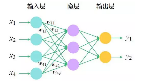
From the literal “deep learningâ€, it can be seen that the neural network has changed its face and returned to the lake. The key lies in a “deep†word. Neural network is a hierarchical model inspired by brain structure. It is composed of a series of nodes connected according to certain rules to form a hierarchical structure. The simplest neural network consists of only three layers: the input layer, the hidden layer (with no direct correlation with the external input and output), and the output layer. Nodes between two adjacent layers are connected by a directed edge, where each edge Correspondence has a weight.
 Â Â
 Â
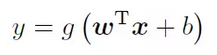
To illustrate the function represented by the neural network, we consider a simpler structure: there is only one input layer and one output layer, where the input layer has d nodes and the output layer has only one node. This node is connected to all input layer nodes. . The input layer node accepts the input x = (x1, x2, · · ·, xd) externally, and the weight corresponding to the connection of the output layer node is w = (w1, w2, · · ·, wd), the output layer node Will make a transformation g of its own input to get the output y, then there is

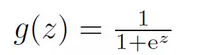
Where the transformation g is usually called the activation function of the node, it is a nonlinear function, such as
Usually we also add a bias item b when summing.
Similarly, we can write the functions represented by the 3-layer neural network
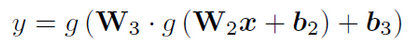
W2 and W3 are the matrices formed by the weights of the connections between the input layer nodes and the hidden layer nodes, the hidden layer nodes and the output layer nodes, and b2 and b3 are the vectors formed by the corresponding offset terms. . By analogy, we can generalize to n-layer neural networks. It can be seen that the neural network has a very large feature that is the introduction of nonlinear activation functions and layer nesting, which makes it possible to represent a highly nonlinear (relative to the input) function, and thus for complex data changes The model has stronger modeling capabilities.
Early neural networks generally had fewer layers (such as the three-layer shallow network) because multi-layered deep networks were difficult to learn and could not perform satisfactorily on various tasks until 2006. be broken. In 2006, Prof. Geoffrey E. Hinton, a master of machine learning, published a paper titled "Reducing the Dimensionality of Data with Neural Networks" in the journal Science. This work provided an effective method for learning deeper networks. The solution: Unsupervised layer-by-layer pre-training of the network opens the door to learning deeper networks. In the next few years, people’s enthusiasm for deep networks has soared to the point where all kinds of problems related to the design and learning of deep networks have been solved, from initialization methods to optimization methods, from activation functions to network structures. Researchers have produced a full range of research on this, allowing deep network training to be done quickly and well. Since the discussion of the neural network itself is not within the scope of this article, it will not be discussed here. The reader only needs to think of the neural network as a model with stronger nonlinear modeling ability.
There are many kinds of neural networks. The above mentioned ones are just the simplest ones. Feedforward neural networks are often also referred to as neural networks. Therefore, the name neural network often refers to only feedforward networks. In the field of computer vision, one of the most successful neural networks is Convolutional Neural Networks (CNN). Its greatest feature is the introduction of convolution operations, replacing full links in feedforward networks with local connections, and in different connections. Sharing weights between them – When a convolution kernel is applied to an image, the convolution kernel is like the observation window at the time of detection. It slides from the upper left corner of the image to the lower right corner. Each position of the sliding corresponds to In an output node, this node is only connected to the input node in the window (each point on the image corresponds to an input node), and the weights of the connection between the different output nodes and the corresponding input node are the same.
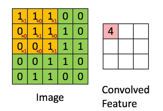
Convolutional neural networks have a unique advantage in dealing with image problems, because the convolution operation can naturally retain the spatial information of the image. It only covers the scope of the local, so the spatial structure of the output node corresponds to the spatial structure of the input node. Feedforward neural networks cannot do this: the order of the input nodes can even be arbitrary, as long as the weights of the connections are exchanged accordingly, the output remains unchanged. CNN was designed by Yann LeCun, a well-known machine learning researcher, as early as the end of the last century, and applied to the recognition of handwritten digits. However, its large-scale application in the field of computer vision originated in 2012 CNN's general task of image classification. Great success.
R-CNN Series
At the end of 2013, deep learning triggered a fire for the target detection task. This kind of fire is R-CNN, where R corresponds to “Regionâ€, meaning that CNN takes the image area as input, and this work eventually develops into A series also inspired and derived a lot of follow-up work. This fire just burned half of the computer vision field.
R-CNN's proposal has revolutionized many of the old practices of the target detection method, and at the same time it has improved the detection accuracy on the standard target detection measurement data set. Changes in the detection method, the first is to abandon the sliding window paradigm, replaced by a new generation of candidate window. For a given image, instead of scanning the image with a sliding window, enumerating all possible scenarios, some sort of candidate window is “nominated†in some way to obtain an acceptable recall rate for the target to be detected. Under the premise, the number of candidate windows can be controlled to several thousand or several hundred. In a sense, multiple classifiers in the VJ face detector are cascaded. Each classifier classifies the candidate window for the next classifier, but this is the same as that used by R-CNN. There is an important difference in the way the candidate window is: In fact, all windows are still checked once, but they are constantly being eliminated. This is a subtraction scheme. In contrast, the candidate window generation method adopted by R-CNN is based on the characteristics of the image to guess where there may be a target to be detected, and how large these goals are. This is a plus from scratch. French program. Selective Search is a typical candidate window generation method, which adopts the idea of ​​image segmentation. Simply put, Selective Search method first divides the image into multiple small blocks based on various color features, and then from the bottom up to the different The blocks are merged. In this process, each block before and after the merging corresponds to a candidate window. Finally, the window most likely to contain the target to be detected is selected as a candidate window.
In addition to the introduction of the candidate window generation method, the second major change is in feature extraction: Artificial features are no longer used, but features are automatically learned using CNN. The feature extraction process is the process of transforming from the original input image (matrix composed of pixel color values) to the feature vector. Previously, Haar features were designed by scientific researchers based on their own experience and knowledge of the research object, in other words, artificial A transformation is defined, and the new approach is to limit only this transformation to CNN--in fact, CNN can already represent enough and complex enough transformations without specific design feature extraction details, replacing training data with human Character. This automatic learning feature is a very distinctive feature of deep learning. Automatically learn the appropriate features. The benefits of this approach are similar to the benefits of allowing the classifier to automatically learn its own parameters. This not only avoids manual intervention, frees up manpower, but also facilitates learning that is more in line with actual data and goals. Features, the two aspects of feature extraction and classification can promote each other and complement each other; but there are also drawbacks, the characteristics of automatic learning are often poor interpretation, can not make people intuitively understand why it would be better to extract features, The other is a certain degree of dependence on training rallies.
It is also worth mentioning that R-CNN introduced a new link in the inspection process: Border Regression (Friendship Reminder: "Box" reads fourth, not polyphonic!), Detection is no longer just a classification. The problem, it is still a regression problem - the difference between regression and classification is that the output of the regression model is not a discrete category label, but a continuous real value. Bounding regression refers to predicting the position and size of the real detection frame on the basis of a given window. That is, if there is a candidate window, if it is discriminated as a personal face window, it will be further adjusted to obtain More precise position and size - better fit to the target to be detected. The frame return provides a new perspective on the one hand to define the detection task, on the other hand it has a more significant effect on improving the accuracy of the test results.
The process of target detection using R-CNN is: firstly use a method such as Selective Search to generate a candidate window, then use the learned CNN to extract the corresponding features of the candidate window, and then the training classifier classifies the candidate window based on the extracted features. The window that is identified as a face is corrected by using a border regression.
Although R-CNN brings about a huge improvement in target detection accuracy, the detection speed is very slow because of the high computational complexity of the candidate window generation method and the depth network used. In order to solve the speed problem of R-CNN, Fast R-CNN and Faster R-CNN appeared. It can be seen from the name that they are faster than one. The first step of acceleration is to use a strategy similar to the integral graph in the VJ face detector. The integral graph is calculated corresponding to the entire input image. It is like a table. When extracting the features of a single window, it directly looks up the table. To obtain the required data, and then perform a simple calculation, each candidate window in the R-CNN needs to use CNN alone to extract features. When there is overlap between the two windows, the overlap is actually repeated. Calculated twice, while in Fast R-CNN, the entire image is taken as input, and the convolution map corresponding to the entire graph is obtained first. Then for each candidate window, the entire map is directly extracted when the features are extracted. The convolutional feature map removes the corresponding area of ​​the window to avoid double counting, and then only needs to scale all the areas to the same size through the so-called RoIPooling layer. The use of this strategy can provide tens or even hundreds of times. Acceleration. In the second step, Fast R-CNN uses a matrix decomposition technique called SVD. Its role is to disassemble a large matrix (approximate) into a product of three small matrices, making the three matrices disassembled. The number of elements is much smaller than the number of elements of the original large matrix, so as to achieve the purpose of reducing the amount of calculation when calculating the matrix multiplication. By applying SVD to the weight matrix of the full connected layer, the time required to process a picture can be reduced by 30%. .

In the third step of acceleration, Faster R-CNN began to focus on the process of generating candidate windows. It used CNN to generate candidate windows, and allowed it to share the convolutional layer with the CNN used for classification and border regression so that the two steps could Use the same convolution map to greatly reduce the amount of calculations.

In addition to using various strategies to accelerate, from R-CNN to Faster R-CNN, the detection framework and network structure are constantly changing. R-CNN does not differ from traditional detection methods in terms of the overall framework. Different links are implemented by separate modules: one module generates a candidate search (Selective Search), one module performs feature extraction (CNN), and one module pair. Window classification (SVM), in addition to adding a module to do border regression. When we went to Fast R-CNN, the last three modules were combined into one module, all of which were done using CNN, so the entire system actually had only two modules left: one module generated a candidate window, and the other module directly performed the window. Classification and correction. Then to Faster R-CNN, all the modules are integrated into a CNN to form an end-to-end framework: the final test result is obtained directly from the input image through a model. This multi-task is in the same model. The common learning approach can effectively use the correlation between tasks to achieve complementary and complementary effects. From R-CNN to Faster R-CNN, this is a zero-smoothing process. The reason for its success is that it benefits from CNN's powerful non-linear modeling capabilities and can learn to fit various subtasks. The feature, on the other hand, is because the perspectives of people's understanding and thinking about the detection problem are constantly changing, breaking the framework of the old sliding window, and viewing the detection as a regression problem and the coupling between different tasks. Although Faster R-CNN is still unable to compare speed with detectors that use non-deep learning methods, with the continuous improvement of hardware computing capabilities and the emergence of new CNN acceleration strategies, the speed issue will surely be able to reach in the near future. has been solved.
Full Convolution Network and DenseBox
Convolutional layer is an essential characteristic of CNN from other types of neural networks. However, CNN usually includes not only convolutional layers, but also full-connection layers. The disadvantage of full-connection layer is that it will destroy the spatial structure of images. So people began to use the convolutional layer to "replace" the full connection layer, usually using a 1 × 1 convolution kernel. This kind of CNN that does not include a fully connected layer is called a full convolutional network (FCN). FCN was originally used for image segmentation tasks, and then it began to be applied to various problems in the field of computer vision. In fact, the CNN used to generate candidate windows in Faster R-CNN is an FCN.
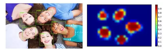
The FCN is characterized by the fact that the input and output are both two-dimensional images, and the output and input have corresponding spatial structures. In this case, we can regard the output of the FCN as a heat map and indicate it with heat. The position of the target to be detected and the covered area: the higher heat is displayed in the area where the target is located, and the lower temperature is displayed in the background area, which can also be seen as performing for each pixel on the image. Classification: Whether this point is on the target to be detected. DenseBox is a typical target detector based on full convolutional network. It obtains the heat map of the target to be detected through FCN, and then obtains the position and size of the target according to the heat map. This provides a new problem for target detection. Solutions. (The following picture is actually derived from another paper. It is used here only to help the reader understand what the face heat map looks like.)
In the DenseBox, it is worth mentioning that while classifying it, it also predicts the location of feature points. Like the JointCascade mentioned in the previous section, DenseBox integrates the two tasks of detection and feature point positioning in the same The location of each point is determined in the network and also by way of a heat map.
CNN-based face detector
The above-mentioned are all common target detectors. These detectors can directly learn face images to obtain face detectors. Although they do not consider the particularity of the human face itself, they can also achieve very good precision. This reflects that the detection of different types of targets is in fact consistent, and there is a common set of mechanisms to deal with target detection problems. There is also a part of the work is specifically for face detection tasks, some consider the characteristics of the face itself, and some are actually more common target detection methods, can naturally migrate to the detection tasks of various types of targets.
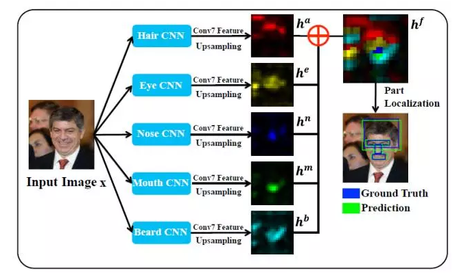
FacenessNet is a detector designed specifically for people's faces. It considers five facial features: hair, eyes, nose, mouth, and moustache. Simply put, for a candidate window, FacenessNet first analyzes the existence of these five parts. Then further judge whether it is a face.
 Â Â
 Â
This method uses both global and local information on the one hand, and can characterize the image content from different perspectives, making the face and non-human faces better differentiated; on the other hand, it enhances the robustness to occlusion. The partial occlusion of the face will affect the overall displayed features, but it will not affect all the local regions, thus enhancing the detector's tolerance to occlusion.
Great leap forward in detection accuracy
As more and more detectors begin to use deep networks, the accuracy of face detection begins to increase dramatically. In 2014, the best detection accuracy achieved by the academic community on the FDDB was a detection rate of 84% with 100 false detections. The accuracy of this accuracy is the JointCascade face detector. By 2015, this record was broken by FacenessNet. With 100 false positives, the detection rate was close to 88%, an increase of almost 4 percentage points. Not only that, the industry's best record has reached a detection rate of 92.5% for 100 false positives, and more than 90% of companies have detected more than one, and these results are based on deep-network-based face detectors. acquired.
While significantly improving the accuracy of face detection, deep learning actually reduces the threshold of various target detection technologies including face detection technology, and it is almost as simple as using deep networks to obtain good detection accuracy; In terms of accuracy, compared to detectors based on non-deep learning methods, detectors based on deep learning methods have to be higher at the starting point. However, in terms of detection speed, detectors based on deep learning methods are still difficult to meet practical application requirements. Even on GPUs, they cannot run at real-time speeds (25fps); on the contrary, once the speed problem can be solved , then deep learning will certainly have broader and more extensive applications for target detection tasks.
| The combination of traditional face detection technology and CNN
Since its introduction, VJ face detector has inspired and influenced a large amount of subsequent work. The integrated graph, AdaBoost method, and cascade structure introduced so far are still used in various forms in various detectors. The traditional face detection technology is superior in speed, but in accuracy it is slightly less than in depth network-based methods. In this case, a natural idea is: whether it can be the traditional face detection technology and deep network. (For example, CNN) to further improve the accuracy under the condition of ensuring the detection speed?
Cascade CNN can be considered as a representative combination of traditional technology and in-depth network. Like VJ face detector, it contains multiple classifiers. These classifiers are organized in a cascade structure, but the difference lies in Cascade CNN. Using CNN as a classifier at each level, rather than using AdaBoost method to combine strong classifiers formed by multiple weak classifiers, and there is no longer a single feature extraction process. Feature extraction and classification are all done by CNN. In the detection process, Cascade CNN adopts the traditional sliding window paradigm. In order to avoid excessive calculation overhead, the first-level CNN contains only one convolutional layer and one full-connection layer, and the size of the input image is controlled at 1212. At the same time, the step size of the sliding window is set to 4 pixels. In this case, on the one hand, the number of candidate windows on each image becomes smaller, and the number of windows decreases according to the square law as the sliding step length increases. On the one hand, the computational cost of extracting features and classifications for each window is also strictly controlled. After the first level of CNN, the second level CNN increases the size of the input image to 2424 due to the more indistinguishable between the face and non-face windows in the passing window to take advantage of more information and improve Network complexity - Although still containing only one convolutional layer and one fully connected layer, the convolutional layer has more convolution kernels, and the full-connection layer has more nodes. The third-level CNN also uses a similar idea to increase the size of the input image while increasing the complexity of the network - using two convolutional layers and a fully connected layer. With the introduction of CNN, the traditional cascaded structure also glows with new brilliance. On the FDDB, Cascade CNN achieved an 85% detection rate when generating 100 false positives, and in the speed, for a size of 640,480 images. With the limited detectable minimum face size of 8080, the Cascade CNN can maintain a processing speed of approximately 10 fps on the CPU. Cascade CNN also uses some other techniques to ensure the accuracy and speed of the detection, such as multi-scale fusion, border calibration, non-maximal suppression, etc. Due to space limitations, it will not be continued here.
Drawing on the essence of traditional face detection technology, drawing on the latest achievements of deep learning research, and exploring and understanding the problems, the search for the best mode of old bottled new wine is a path that is worth continuing to explore.
| Simple thinking about the status quo and the future
After decades of research and development, face detection methods are maturing, and they have been widely used in real-life scenarios. However, face detection problems have not yet been completely resolved, and complex and diverse posture changes have been bizarre. Occlusion, unpredictable lighting conditions, different resolutions, unclear sharpness, subtle skin color differences, and various internal and external factors work together to make the face change pattern extremely rich. At present, there are no detectors that can simultaneously It is robust enough to all change modes.
Current face detectors have been able to achieve good performance on FDDB. Many detectors have detected more than 80% of the 100 false positives, which means that they detect more than 40 faces. A false positive. So far, the false detection and recall rates mentioned in this article correspond to discrete ROC curves on FDDB. The term “discrete†refers to whether each face is detected with 1 and 0 respectively. Correspondingly, there is also a continuous score ROC curve, and “continuous type†refers to whether the face is detected or not by means of the ratio of the intersection between the detection frame and the markup frame, and in a sense, continuous The type score attempts to judge the accuracy of the detection frame, that is, the position and size of the detection frame is close to the actual face's position and size. For two different detectors, the relative relationship between the two types of curves is not exactly the same: two detectors with discrete ROC curves close to each other, and their corresponding continuous ROC curves may have significant differences. Most directly, this shows that although some detectors detect human faces, but the accuracy of the detection frame is relatively low, but in fact another important reason for this inconsistency lies in the difference between the detection frame and the label frame. . In the FDDB, faces are marked by ellipses. In most cases, the entire head is included. In contrast, the detector gives a detection result that is a rectangular face frame and usually contains only the face. Zones—especially for detectors that use the sliding window paradigm, this can easily cause the crossover ratio between the detection frame and the marked ellipse to be too small, perhaps even less than 0.5. For different detectors, the size of the box corresponding to the situation that can best distinguish the face from the non-human face window will be different, so that the detection frame given by different detectors will also be different. The method of expanding the detection frame or returning to the ellipse will be adopted to minimize the influence caused by the inconsistency between the labeling frame and the detection frame, and ensure the fairness of the evaluation.
In addition to the question of the markup frame, to view the evaluation results on the FDDB more objectively, we need to consider another point: the difference between face and actual application scenarios on the FDDB test image. In other words, we need to think about such a problem. : Can the accuracy achieved by the face detector on the FDDB truly reflect its performance in practical application scenarios? The face of the test image in the FDDB includes changes from expressions to poses, from illumination to occlusion, and is thus a relatively general data set. However, in practical applications, faces are often more distinctive in different scenes. The characteristics, such as in the video surveillance scene, due to the high camera mounting position and limited resolution, and the introduction of noise in the storage and transmission process, the face of the image tends to have a larger pitch angle, and the definition is relatively Low, in this case, a detector that performed excellently on FDDB may not necessarily achieve satisfactory accuracy. In the FDDB, about 10% of human faces are under 4040 in size, and for some tasks such as face recognition, too small human faces are not suitable, so if a detector performs poorly on a small face And it causes it to be flat on the FDDB, but there are not much differences between the larger face and some of the better performing detectors. Applying it to face recognition tasks is completely problem-free. It may even be because The simplicity of the model brings speed advantages. In short, when faced with specific application scenarios, on the one hand, we still need specific analysis of specific issues, we can not blindly determine the accuracy of the detector on FDDB or other face detection data sets; on the other hand, we need to The current face detector adapts the actual data to be processed so that the detector can achieve better accuracy in a specific scene.
In addition to FDDB, the more commonly used set of face detection evaluations are AFW, and MALF, IJB-A, and Wider Face that have been disclosed in recent years. AFW contains a relatively small number of images, a total of only 205 test images, annotated 468 faces, but because it covers a large number of face change patterns, it is a certain degree of challenge, it is also more commonly used. The other three evaluation sets are relatively large in image size. MALF and Wider Face do not publish face recognition and evaluation programs. They need to submit test results to the publisher for evaluation. This prevents, to some extent, the inconsistency of evaluation methods. This results in unfairness and overfitting of the test set; the two data sets also divide the test set into multiple subsets according to different attributes (such as resolution, pose, difficulty, etc.) Tests are performed on the full set and subset, which can more fully reflect the detector's ability in different scenarios. IJB-A contains not only static face images but also video frames extracted from video. In all the evaluation sets mentioned above, only Wider Face provides specialized training sets and verification sets. Other evaluation sets only contain test sets. This actually brings a problem to the comparison of different methods: we have difficulty judging the cause of detection. The reason why there is a difference in the accuracy of the instrument is whether it is training data or the algorithm and the model itself, and it is not known whether those two factors play a greater role. Wider Face should be the most difficult evaluation set. The marked faces have very large spans in terms of posture and occlusion, and the face with a resolution below 5050 accounts for 50% (the training set and the checksum have reached More than 80%), but in some application scenarios (such as face recognition), it is not necessary to care too much about a small-sized face.
Although deep-network-based detectors can currently achieve high detection accuracy, and their versatility is very strong, the computational cost they pay is also very high. Therefore, the key to the breakthrough of such detectors lies in the simplification and acceleration of deep networks. In addition, if face detection alone is considered, this classification problem is relatively simple, and there is a possibility that learning a small network directly can do this task well enough. For detectors that use non-deep learning methods, the basic detection accuracy will be much lower than that of the detectors, but there will be obvious advantages in speed, so the key is to make reasonable improvements and adaptations to the problems in specific application scenarios. For better detection accuracy.
In order to provide a more convenient human-computer interaction interface, create effective visual understanding means, let the machine become warm, observe, feel, the vast number of scientific research workers are still exploring the face detection and general target detection tasks. . One day, when we face each other with the machine, we can smile each other: science makes life better!
postscript
This paper begins with the face detection task itself, introduces the general flow of face detection, and then introduces three different types of face detection methods: the traditional method represented by the VJ face detector, and the modern method based on the depth network. And a combination of traditional face detection technology and deep network. However, in the course of decades of face detection, there are many other methods that cannot be attributed to these three categories, of which the more important ones are based on component model-based methods and model-based methods, although this article does not Two methods are introduced, but they still have important status and significance in the face detection problem. Interested readers can further read related papers to understand.
Lei Feng Network (search "Lei Feng Net" public concern) (search "Lei Feng Net" public concern) Note: This article was published by the author in the Deep Learning Lecture, reproduced please contact the authorizing and retain the source and author, not to delete the content.
Half-cut Cells Mono Solar Panel
Half-cut cells mono solar panel
Half-cut cells mono solar panel
Zhejiang G&P New Energy Technology Co.,Ltd , https://www.solarpanelgp.com